Data science: Google Analytics and R programming

THE TRADITIONAL FUNCTIONS OF MEASUREMENT TOOLS IN ANALYTICS

Over the years, measurement tools in analytics have become ubiquitous. In fact, it is now very rare that a website does not use any of them. We find Google Analytics at the forefront, which has enjoyed strong adoption thanks to the performance and the free nature of its solutions. Many marketers frequently use this data to guide their marketing decisions or to check the performance of campaigns, for example.

When a marketer thinks of a measurement tool, they probably have graphs and charts in mind that help to better understand consumer behavior. However, behind these charts and graphs is an innumerable amount of data collected by these tools! This data is generally made available via API by service providers, such as Google Analytics and Adobe Analytics , to name a few.

This access to raw data is of great value for organizations since it can better answer important questions in marketing such as sales forecasting for example. Indeed, many of these questions cannot be answered directly using a measurement tool. This is when data processing using statistical programming tools and languages comes into its own.

WHAT CAN BE ACCOMPLISHED WITH ANALYTICS DATA IN STATISTICAL PROGRAMMING?

In this article, two use cases will be put forward: the first case that I propose to you is that of forecasting ( forecasting ) sessions on a website. The second will present a visitor segmentation approach based on user browsing data. For those interested, the complete R code to reproduce the examples that will follow is available at the end of the article.

For information purposes, the data used in this context comes from Google Analytics and will be processed using the R programming language for its strong statistical analysis capabilities. Note that the analysis can also be done with Adobe Analytics or Segment, for example.

1. FORECASTING SESSIONS ON A WEBSITE

To enable the creation of a time series forecasting model, you must first generate a data file. To do this, several R packages to directly collect the available data. I recommend the use of googleAnalyticsR by Mark Edmondson .

Once you have your data file, you can start a data visualization process, which will allow you to better understand the evolution of sessions on your website.

R CODE TO CREATE YOUR DATA FILE

library(googleAnalyticsR)
View_id <- XXXXXXXX # Le view ID est situé dans votre compte Google Analytics
date_debut_forecast <- "2013-01-01" 
date_fin_forecast <- "2018-12-31"
metriques_forecast <- c("ga:sessions")
dimensions_forecast <- c("ga:yearmonth")

# Appel à Google Analytics pour la création du fichier de données
ga_forecast <- google_analytics(view_id, date_range = c(date_debut_forecast, date_fin_forecast), 
                                metrics = metriques_forecast, 
                                dimensions = dimensions_forecast)

# Formatage du data.frame en time series
ga_forecast1 <- dcast(ga_forecast, 
                      yearmonth ~ ., 
                      value.var = "sessions")
rownames(ga_forecast1) <- ga_forecast1$yearmonth
ga_forecast1$yearmonth = NULL
ga_forecast2 <- ts(ga_forecast1, frequency=12)

# Visualisation des sessions sur le site web
plot(ga_forecast2)

SESSION ON THE SITE IN THE LAST 7 YEARS

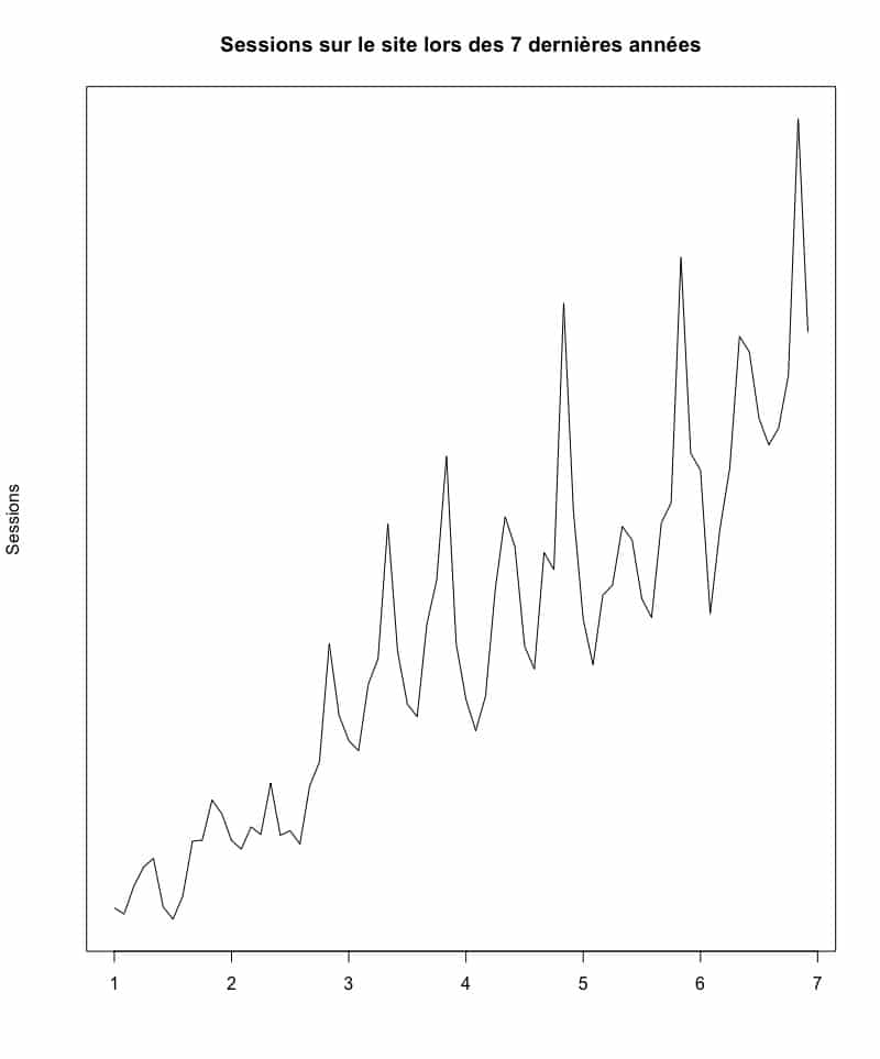
By analyzing the graph above, we first notice that the number of sessions seems to have experienced a constant evolution in the last seven years. In other words, it seems that the session growth trend is constantly on the rise. You will be able to notice peaks and valleys quite distinctly at regular intervals in the evolution of the sessions. One could therefore deduce that there is a certain seasonality in the sessions on this website. You can do trend and seasonality analysis accurately using a method of decomposing our time series. With the help of a few lines of R code, you will be able to analyze the decomposition.

R CODE TO DECOMPOSE YOUR TIME SERIES

# Décomposition de la série en tendance et saisonnalité
forecast_decomp <- decompose(ga_forecast2)
plot(forecast_decomp)

BREAKING DOWN OUR TIME SERIES

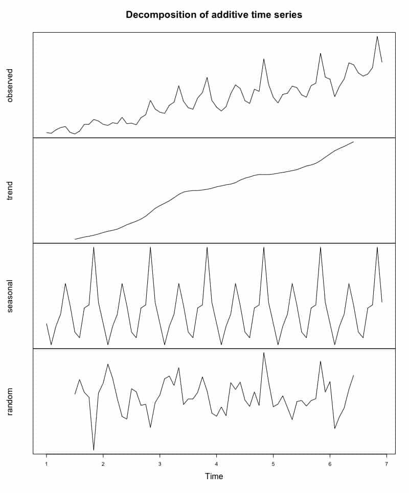
Our reading of the situation was therefore correct:

Indeed, by looking at the second curve, that of the trend, we can confirm that it has been relatively constant over the past seven years.
As for the third curve, there is a strong seasonality that is easy to identify. In this case, it seems that May and November are good months in terms of sessions on this website. Conversely, the months of February and July are the months with a consistently lower number of sessions compared to the other months of the same year.

Now that you have a better understanding of the time series and the data, you can create a session forecast model for future years. The R package called " forecast ", created by Australian statistician Rob J. Hyndman , makes it easy to create a time-series forecast model as well as to visualize this forecast on a graph. Here is an example of forecasting sessions on a website for the next two years.

R CODE FOR FORECASTING

# Forecasting des sessions sur le site web
ga_forecast3 <- msts(ga_forecast2, seasonal.periods = c(12))
forecasting <- tbats(ga_forecast3)
forecasting2 <- forecast(forecasting)
plot(forecasting2)

FORECAST OF SESSIONS ON THE SITE OVER THE NEXT TWO YEARS

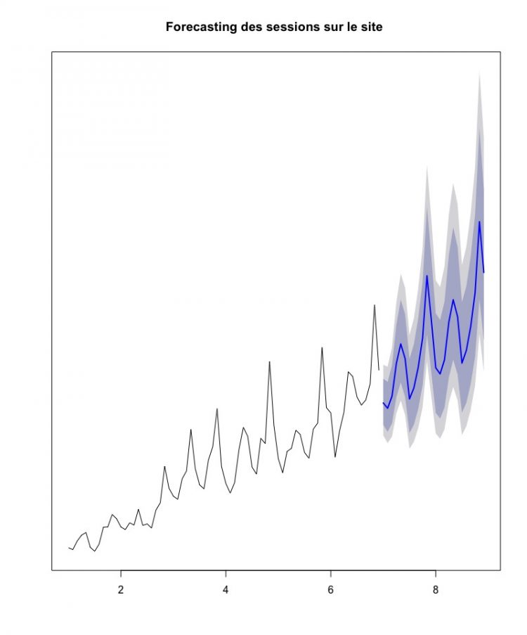
The blue line represents the forecast, while the colored areas represent the confidence interval (80% dark and 95% light) of our forecast model. If our model is correct, it looks like sessions will continue to grow for the next few years.

2. UNSUPERVISED SEGMENTATION

Companies generally have a certain definition of their targets, even that many use personas to make their definition more concrete. One of the potential limitations of personas stems from the fact that it is often a more or less arbitrary interpretation of who our target is. To add a certain level of precision, there are also statistical tools which make it possible to calculate the homogeneity of a group of individuals by taking variables into account. To achieve this, I suggest that you use the browsing data of a site to try to define browsing groups there in a similar way.

As in the first use case, you will have to start by creating the data file. To do this, you will need to start by collecting navigation data from your site's users over a period of one year. You can use several variables and experiment to find out which variables are the most relevant. For example purposes, here are the variables I will use in this case:

number of sessions in a year,
the number of hits ,
the number of page views,
the number of product page views,
the average time spent on a page,
the number of transactions,
the average duration of the sessions,
the bounce number,
the average number of page views per session.

The first thing you'll want to see is if adding segments tends to make your groups more homogeneous . To achieve this, pay attention to your grouping analysis. You're really trying to find a balance between precision and ease of interpretation. Following the creation of the data file and the analysis of the sum of the errors, you will obtain the graph following the block of code below.

R CODE TO CREATE A DATA FILE FOR SEGMENTATION

view_id <- XXXXXXXX

date_debut <- "2018-01-01"
date_fin <- "2018-12-31"
metriques_segmentation <- c("ga:sessions", "ga:hits", "ga:pageviews","ga:productDetailViews", "ga:timeOnPage", "ga:transactions", "ga:sessionDuration","ga:bounces", "ga:pageviewsPerSession")
dimensions_segmentation <- c("ga:dimension10")

# Call to Google Analytics
ga_segmentation <- google_analytics(view_id, date_range = c(date_debut, date_fin), metrics = metriques_segmentation, dimensions = dimensions_segmentation)

# Preparation of the data file for segmentation analysis
segmentation <- na.omit(ga_segmentation)
segmentation2 <- scale(segmentation1)

# Identify the number of segments
within_sum_square <- (nrow(segmentation2)-1)*sum(apply(segmentation2,2,var))
for (i in 2:15) within_sum_square[i] <- sum(kmeans(segmentation2, centers=i)$withinss)

# Visualization
plot(within_sum_square, type = "b")

SELECTION OF THE NUMBER OF SEGMENTS

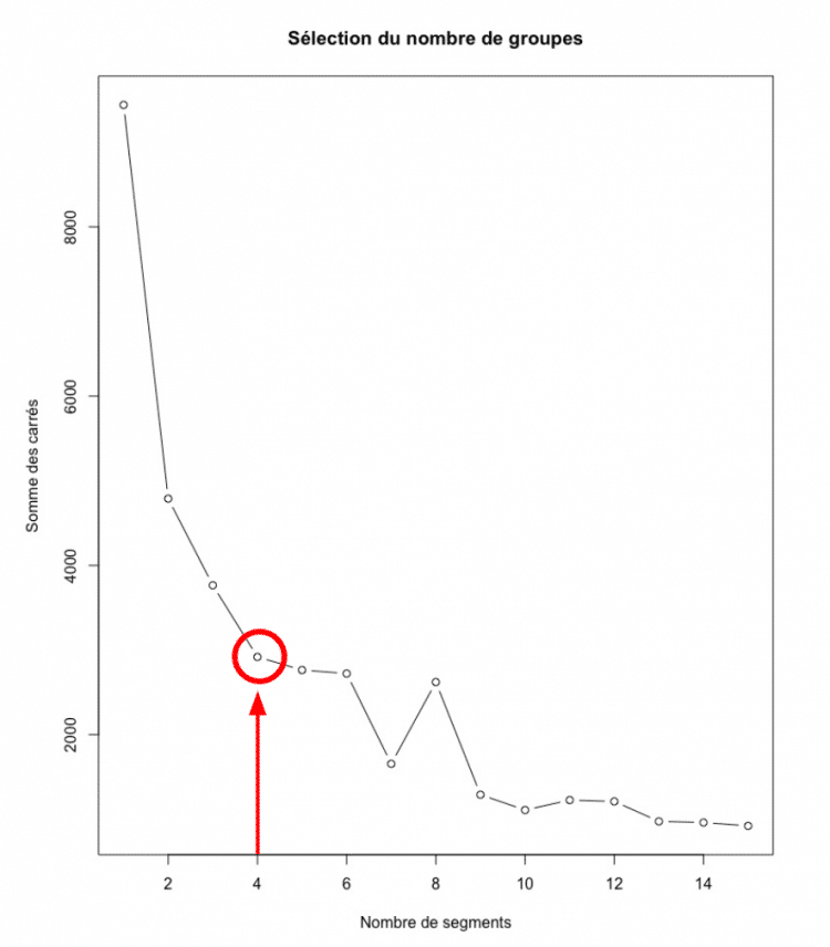
By analyzing the table, you will find that it is after four segments that the reduction in the sum of the squares begins to be less and less significant. These four segments consist of a reasonable number to ensure ease of interpretation. It is for this reason that it would be better to segment your database into four groups. Using a well-known approach, k-means , you can then proceed to segment your database. To validate if the groups seem to make sense, you can also inspect the visualization of the groupings.

R CODE FOR K-MEANS SEGMENTATION

# Segmentation k-means en utilisant la solution des 4 segments identifiés précédemment
kmean_segmentation <- kmeans(segmentation2, 4)
aggregate(segmentation2,by=list(kmean_segmentation$cluster),FUN=mean)
segmentation2 <- data.frame(segmentation2, kmean_segmentation$cluster)

# Visualisation des segments 
clusplot(segmentation2, kmean_segmentation$cluster, color=TRUE, lines=0)

VISUALIZATION OF OUR SEGMENTATION

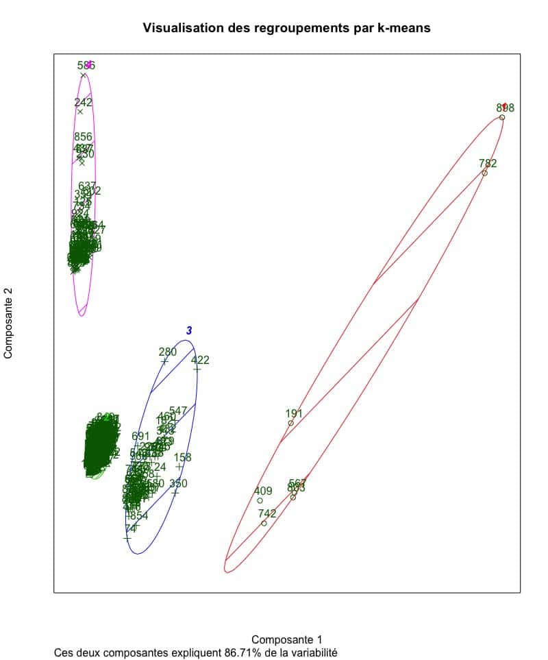
The visualization of the segments created using the navigation data seems to conclude that the four groups are rather homogeneous. In fact, this example captures over 86% of the variability that existed between the points before performing clustering analysis. This is therefore relevant information to draw a portrait of users visiting a website or to better understand the context and browsing habits.

This kind of approach can also serve as a starting point in a persona creation process. The mixed search methods used by Adviso in CX, for example, take advantage of unsupervised segmentation methods such as the one demonstrated above.

By presenting two concrete use cases for the use of data that you probably already have, I hope I have convinced you that the exploitation of data beyond prescribed practices is much easier than you might think. . The Data Science team of which I am a part is constantly looking at issues and opportunities of this kind. Contact us to discuss creative ways to activate your business data!

R CODE USED FOR WRITING THIS ARTICLE

#############################################################
#############################################################
# Analyse des données Google Analytics avec R
#############################################################
#############################################################

#############################################################
# Installation des packages requis
install.packages("googleAnalyticsR")
install.packages("tidyverse")
install.packages("reshape2")
install.packages("cluster")
install.packages("fpc")
install.packages("forecast")

#############################################################
# Initialisation des packages requis
library(googleAnalyticsR)
library(tidyverse)
library(reshape2)
library(cluster)
library(fpc)
library(forecast)

# Authentification pour GA. Ouvrez votre fureteur web pour autoriser
ga_auth()

# Sélection des paramètres
view_id <- XXXXXXXX # Insérez ici à la place des X le ID pour VOS données
date_debut <- "2018-01-01" 
date_fin <- "2018-12-31"
date_debut_forecast <- "2013-01-01" 
date_fin_forecast <- "2018-12-31"
metriques_forecast <- c("ga:sessions")
dimensions_forecast <- c("ga:yearmonth")
metriques_prediction <- c("ga:transactionRevenue", "ga:sessions", "ga:hits", "ga:pageviews","ga:productDetailViews", "ga:timeOnPage", "ga:transactions", "ga:sessionDuration")
dimensions_prediction <- c("ga:dimension10")
metriques_segmentation <- c("ga:sessions", "ga:hits", "ga:pageviews","ga:productDetailViews", "ga:timeOnPage", "ga:transactions", "ga:sessionDuration","ga:bounces", "ga:pageviewsPerSession")
dimensions_segmentation <- c("ga:dimension10")

#############################################################
####### Forecasting des sessions sur un site web ############
#############################################################
# Appel à Google Analytics pour la création du fichier de données
ga_forecast <- google_analytics(view_id, date_range = c(date_debut_forecast, date_fin_forecast), 
                                metrics = metriques_forecast, 
                                dimensions = dimensions_forecast)

# Formatage du data.frame en time series
ga_forecast1 <- dcast(ga_forecast, 
                      yearmonth ~ ., 
                      value.var = "sessions")
rownames(ga_forecast1) <- ga_forecast1$yearmonth
ga_forecast1$yearmonth = NULL
ga_forecast2 <- ts(ga_forecast1, frequency=12)

# Visualisation des sessions sur le site web
plot(ga_forecast2)

# Décomposition de la série en tendance et saisonnalité
forecast_decomp <- decompose(ga_forecast2)
plot(forecast_decomp)

# Forecasting des sessions sur le site web
ga_forecast3 <- msts(ga_forecast2, seasonal.periods = c(12))
forecasting <- tbats(ga_forecast3)
forecasting2 <- (forecast(forecasting))
plot(forecasting2)

#############################################################
############## Segmentation non supervisée ##################
#############################################################
# Appel à Google Analytics
ga_segmentation <- google_analytics(view_id, date_range = c(date_debut, date_fin), 
                                    metrics = metriques_segmentation, dimensions = dimensions_segmentation)

# Préparation du fichier de données pour l'analyse de segmentation
segmentation <- na.omit(ga_segmentation)
segmentation2 <- scale(segmentation1)

# Identifier le nombre de segments
within_sum_square <- (nrow(segmentation2)-1)*sum(apply(segmentation2,2,var))
for (i in 2:15) within_sum_square[i] <- sum(kmeans(segmentation2, centers=i)$withinss)
plot(within_sum_square, type = "b")

# Segmentation k-means en utilisant la solution des 4 segments identifiés précédemment
kmean_segmentation <- kmeans(segmentation2, 4)
aggregate(segmentation2,by=list(kmean_segmentation$cluster),FUN=mean)
segmentation2 <- data.frame(segmentation2, kmean_segmentation$cluster)

# Visualisation des segments 
clusplot(segmentation2, kmean_segmentation$cluster, color=TRUE, lines=0)